[1] 0.1748401 0.6809099Inference and uncertainty quantification
(How to express the fact we do not know the unknown)
Andrew Pua
Previously…
We calculated summaries and linear regressions using whatever data we have on hand.
- We explored how these aspects may be related to each other algebraically.
- We also discussed how to communicate the results.
- We also discovered the behavior of these procedures in the “long run”.
Now…
I discuss the remaining convergence concept called convergence in distribution.
The idea is that if we suitably standardize the random variables associated with our procedures, there is another form of order in the “long run”.
The use of this convergence concept shows up in two typical inference tasks: constructing confidence intervals and testing hypotheses.
I discuss the most crucial ideas in the simplest setting of inference for a common population mean.
After discussing the crucial ideas, we move on to the more general cases encountered in practice and the use of the bootstrap.
Convergence in distribution
- Define the cumulative distribution function (cdf) of \(X\) as \(F_{X}\left(x\right)=\mathbb{P}\left(X\leq x\right)\).
- Let \(Z_1,Z_2,\ldots\) be a sequence of random variables. \(Z_n\) converges in distribution to \(Z\), denoted by \(Z_n\overset{d}{\to}Z\), if \[\lim_{n\to\infty}F_{Z_n}\left(z\right)=F_Z\left(z\right)\] for all points \(z\) at which \(F\) is continuous.
- Some refer to convergence in distribution as convergence in law.
- One reason why we look at the cdf is that it unifies the discrete and continuous cases.
- The convergence concept focuses on the cdfs of the sequence of random variables and NEITHER on the moments of the random variables (recall mean-squared convergence) NOR on the events related to the random variables (recall convergence in probability).
- Why would this concept be useful?
- Typically, we really do not know the actual form of the cdf of \(F_{Z_n}\) for any \(n\).
- But if it happens that we know the actual form of \(F_Z\) (meaning that it is one of those special and named distributions), then convergence in distribution becomes an extremely useful concept!
- In applied work, \(F_Z\) is usually a normal or standard normal cdf.
An example
Let \(X_1,\ldots,X_{50}\) be IID random variables, each having a \(U(0,1)\) distribution.
Your task is to find \(\mathbb{P}\left(\overline{X} \leq 0.4 \right)\).
Note that the example asks you to calculate probabilities involving the sample mean.
But it could have easily been calculating probabilities involving the regression coefficients, say \(\mathbb{P}\left(\left|\widehat{\beta}\right| > 2 \right)\).
The sample mean and the regression coefficients here are really random variables and not any specific sample mean or regression coefficients you have calculated after seeing the data.
- This is an important but often neglected and misunderstood point.
Now, how would you accomplish this task? To find the desired probability, you have many options, depending on the information you exploit.
Use Monte Carlo simulation, but this is an approximation (give or take sampling variation).
- At this stage, you can already do this! If not, then there is a problem.
Find the exact distribution of \(\overline{X}\), then compute the desired probability (up to rounding errors).
- You might not be able to do this, not because you were not taught this but rather finding the exact form of the distribution is extremely challenging. Even the case for \(n=2\) is already complicated.
Determine whether the cdf of \(\overline{X}\) may be approximated by the cdf of some known random variable. Use the latter cdf to provide a large-sample approximation.
- This approach works if you know a central limit theorem.
There is actually another approach which uses a version of the bootstrap, but we will come back to this later.
A central limit theorem (CLT)
- Let \(X_1, X_2,\ldots\) be IID random variables with finite mean \(\mu=\mathbb{E}\left(X_t\right)\) and finite variance \(\sigma^2=\mathsf{Var}\left(X_t\right)\). Then the sequence of sample means \(\overline{X}_1, \overline{X}_2, \ldots\) has the following property: \[\lim_{n\to\infty}\mathbb{P}\left(\frac{\overline{X}_n-\mu}{\sigma/\sqrt{n}} \leq z\right) = \mathbb{P}\left(Z\leq z\right)\] where \(Z\sim N(0,1)\).
- Sometimes we write the previous result as \[\frac{\overline{X}_n-\mu}{\sigma/\sqrt{n}} \overset{d}{\to} N(0,1)\] or \[\sqrt{n}\left(\overline{X}_n-\mu\right) \overset{d}{\to} N\left(0,\sigma^2\right)\]
- The concept of convergence in distribution is featured in another celebrated result in probability theory called the CLT for IID random variables.
How to use the CLT to our example
- Recap: Let \(X_1,\ldots,X_{50}\) be IID random variables, each having a \(U(0,1)\) distribution. Your task is to find \(\mathbb{P}\left(\overline{X}_{50} \leq 0.4 \right)\).
- The setup matches the requirements of the CLT. Here we have \(\mu=1/2\) and \(\sigma^2=1/12\).
- So, we have \[\begin{eqnarray*} \mathbb{P}\left(\overline{X}_{50} \leq 0.4\right) &=& \mathbb{P}\left(\frac{\overline{X}_{50}-\mu}{\sigma/\sqrt{n}} \leq \frac{0.4-\mu}{\sigma/\sqrt{n}}\right) \\ &=&\mathbb{P}\left(\frac{\overline{X}_{50}-\mu}{\sigma/\sqrt{n}} \leq \frac{0.4-1/2}{\sqrt{1/12}/\sqrt{50}}\right) \\ &\approx & \mathbb{P}\left(Z\leq -2.44949\right)\end{eqnarray*}\] where \(Z\sim N(0,1)\).
What if you do not know \(\mu\) and \(\sigma^2\)? In the example, we exploited information from the moments of \(U(0,1)\).
It can be shown that the CLT still holds if a consistent plug-in is used for \(\sigma^2\): \[\frac{\overline{X}_n-\mu}{S_n/\sqrt{n}} \overset{d}{\to} N(0,1)\] Here \(S_n\) is the sample standard deviation where \(S_n\overset{p}{\to} \sigma\).
This means that if you have a random sample on hand, then \(S_n\) can be used as a plug-in for \(\sigma\).
Notice that we cannot use a consistent plug-in for \(\mu\)!!
- Typically, we or others might have claims about \(\mu\). We can use that information as a plug-in for \(\mu\).
- The bootstrap has a way to deal with this, but we come back to this later.
A final thing to note is the following: Actually we are really estimating \(\sigma/\sqrt{n}\) which is the standard error of the sample mean.
Why do we need confidence intervals?
We want to give a statement regarding a set of plausible values (interval or region) such that we can “cover” or “capture” the unknown quantity we want to learn with high probability.
This high probability can be guaranteed under certain conditions. But this is a long run concept applied to the procedure generating the confidence interval.
How to construct a confidence interval
- Actually there are many ways to construct a confidence interval. The most taught way is indirectly via the CLT.
- Our target is to construct a \(100(1-\alpha)\%\) confidence interval for \(\mu\).
- Note that you have to set \(\alpha\) in advance. \(100(1-\alpha)\%\) is called the confidence level.
- The idea is to work backwards:
\[\begin{eqnarray*}\mathbb{P}\left(\overline{X}_n-z\cdot \frac{\sigma}{\sqrt{n}} \leq \mu \leq \overline{X}_n+z\cdot \frac{\sigma}{\sqrt{n}}\right) &=& \mathbb{P}\left(-z \leq \frac{\overline{X}_n-\mu}{\sigma/\sqrt{n}} \leq z\right) \\ &\approx & \mathbb{P}\left(-z\leq Z\leq z\right)\end{eqnarray*}\] where \(Z\sim N(0,1)\).
- By choosing the appropriate \(z\), you can guarantee that \(\mathbb{P}\left(-z\leq Z\leq z\right)=1-\alpha\).
If you do not know the standard error, you have to estimate it. Use a consistent plug-in for the unknown parameter \(\sigma\).
The guarantee still holds:
\[\begin{eqnarray*}\mathbb{P}\left(\overline{X}_n-z\cdot \frac{S_n}{\sqrt{n}} \leq \mu \leq \overline{X}_n+z\cdot \frac{S_n}{\sqrt{n}}\right) &=& \mathbb{P}\left(-z \leq \frac{\overline{X}_n-\mu}{S_n/\sqrt{n}} \leq z\right) \\ &\approx & \mathbb{P}\left(-z\leq Z\leq z\right)\end{eqnarray*}\] where \(Z\sim N(0,1)\).
In practice, \[\left[\overline{X}_n-z\cdot \frac{S_n}{\sqrt{n}} , \overline{X}_n+z\cdot \frac{S_n}{\sqrt{n}}\right]\] with \(z\) properly chosen will give a large-sample confidence interval for \(\mu\).
Note that the confidence interval here is symmetric. It does not have to be. We will see examples that show that these symmetric confidence intervals may not make sense.
A simulation to illustrate confidence intervals
Assume that \(X_1,\ldots, X_5\overset{\mathsf{IID}}{\sim} U\left(0,1\right)\).
In this situation, you do know the common distribution \(U\left(0,1\right)\) and that \(\mu=1/2\) and \(\sigma^2=\mathsf{Var}\left(X_t\right)=1/12\).
Our target is to construct an interval so that we can “capture” \(\mu\) with a guaranteed probability.
- We can check the rate of “capture” because we know everything in the simulation.
Is the true mean \(\mu=1/2\) in the interval?
This is one confidence interval calculated for one sample of size 5.
So where does the “high probability” come in?
- Draw another random sample and repeat the construction of the confidence interval.
[1] 0.2372673 0.7433371Is the true mean \(\mu=1/2\) in the interval?
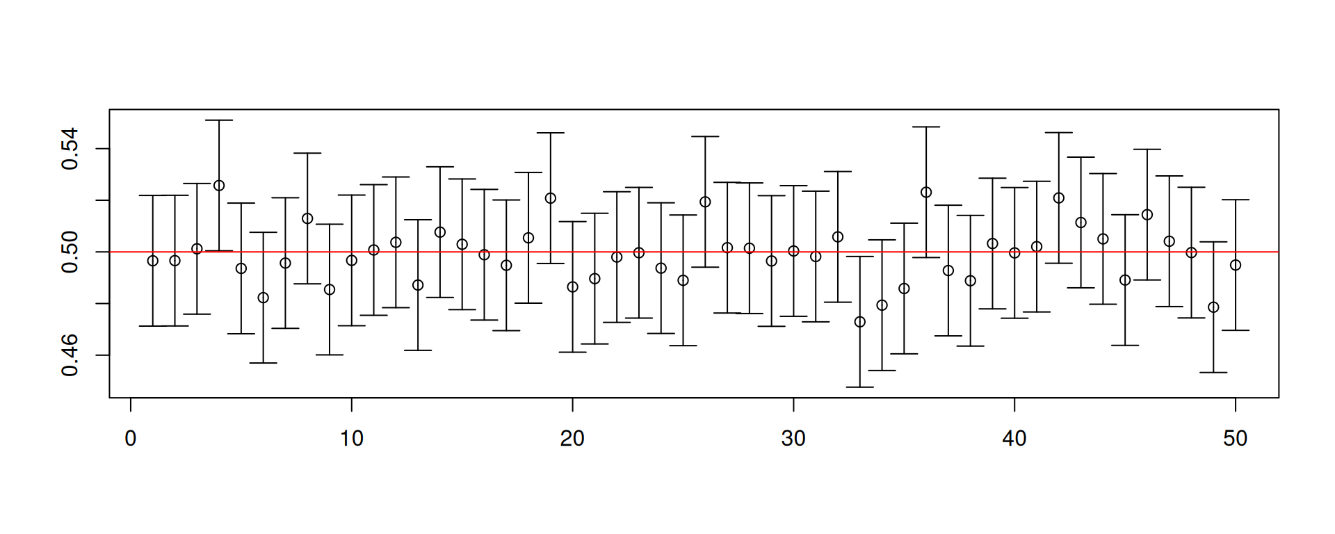
Let us repeat the construction of the confidence interval 10000 times.
cons.ci <- function(n)
{
data <- runif(n)
c(mean(data)-1.96*sqrt(1/12)/sqrt(n), mean(data)+1.96*sqrt(1/12)/sqrt(n))
}
results <- replicate(10^4, cons.ci(5))
mean(results[1,] < 1/2 & 1/2 < results[2,])[1] 0.9508# Increase the number of observations
results <- replicate(10^4, cons.ci(500))
mean(results[1,] < 1/2 & 1/2 < results[2,])
[1] 0.9535- Take note that the standard error was computed based on the known variance.
- To visualize the intervals, you have to install an extra package called
plotrix.
- What happens if you do not know \(\mathsf{Var}\left(X_t\right)\)? You may plug-in a good estimator for it.
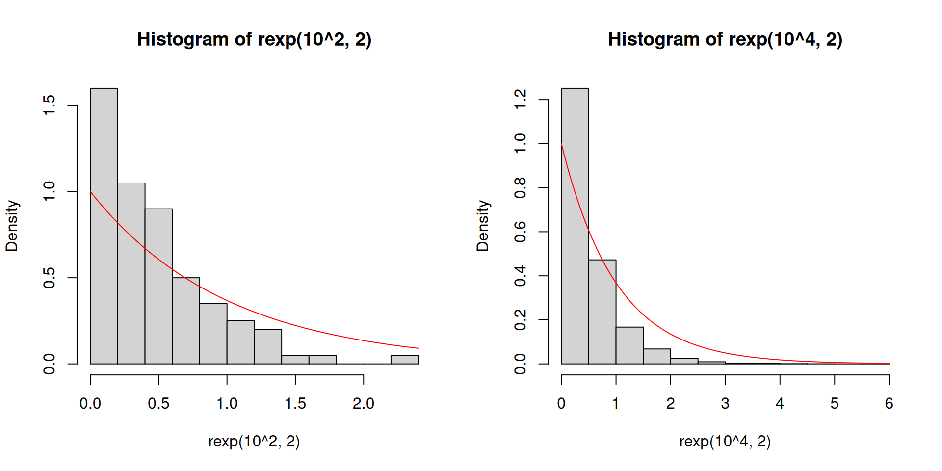
Let us change the distribution to an exponential distribution with rate parameter equal to 2.
Here the population mean is 1/2 and the population variance is 1/4.
This is a skewed distribution, unlike \(U(0,1)\).
You may not have encountered this special distribution but this distribution is special in engineering settings, climate change applications, and sometimes can show up in economics.
- Recall our previous code for constructing 95% confidence intervals for \(\mu\):
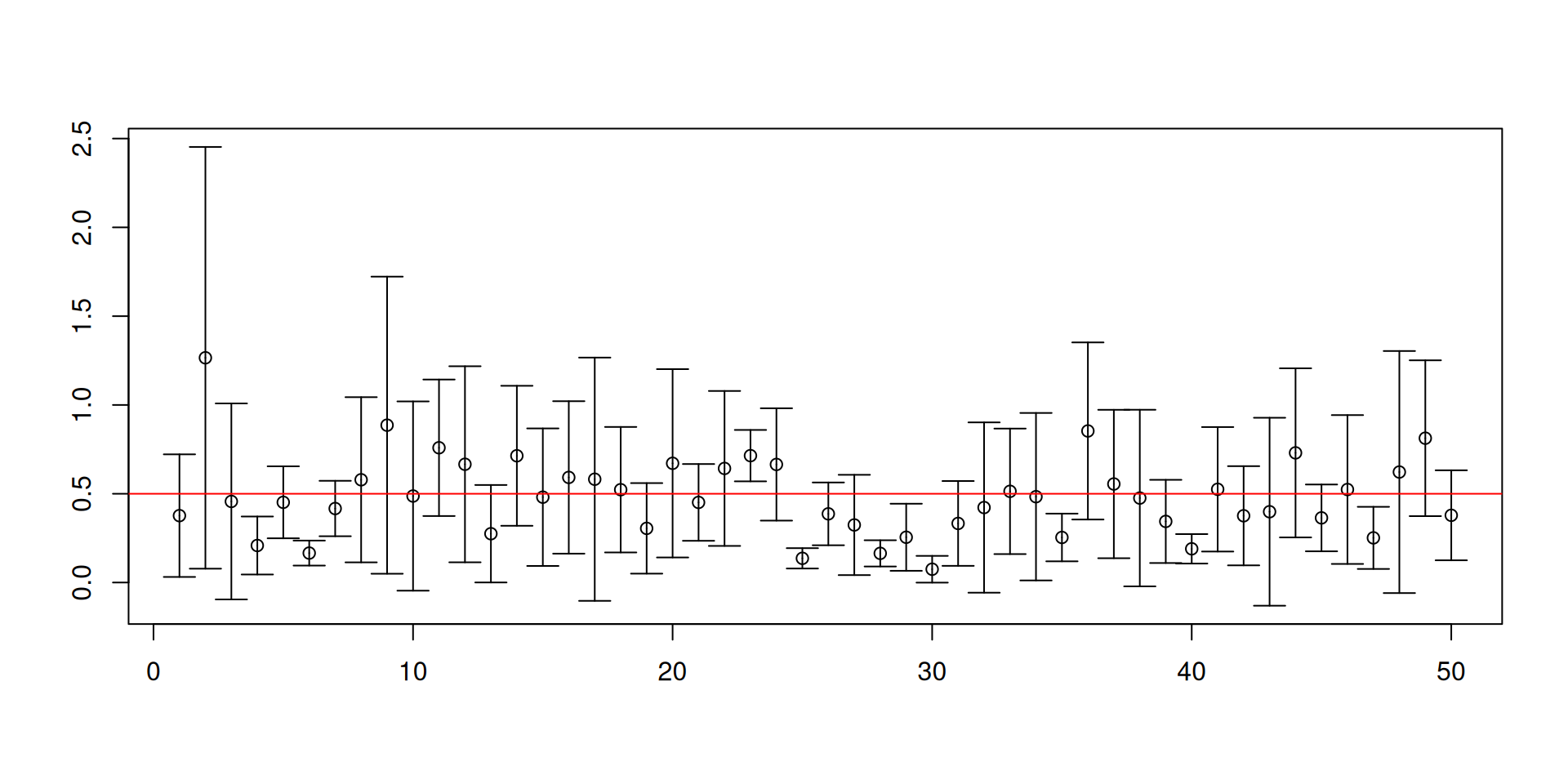
[1] 0.9032[1] 0.0076 0.0892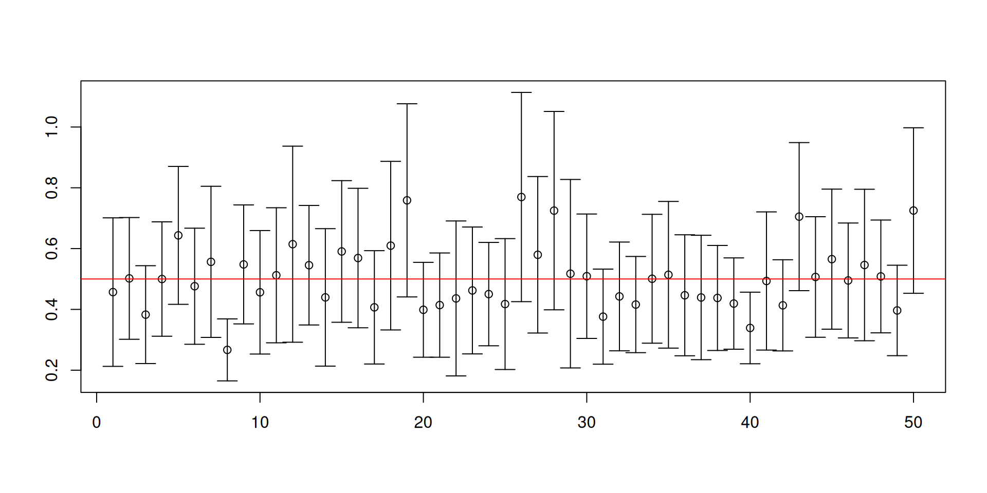
[1] 0.9372[1] 0.0129 0.0499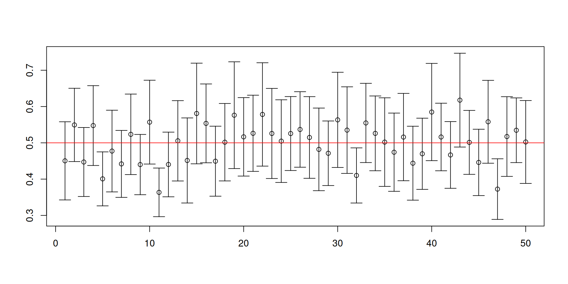
[1] 0.9454[1] 0.0184 0.0362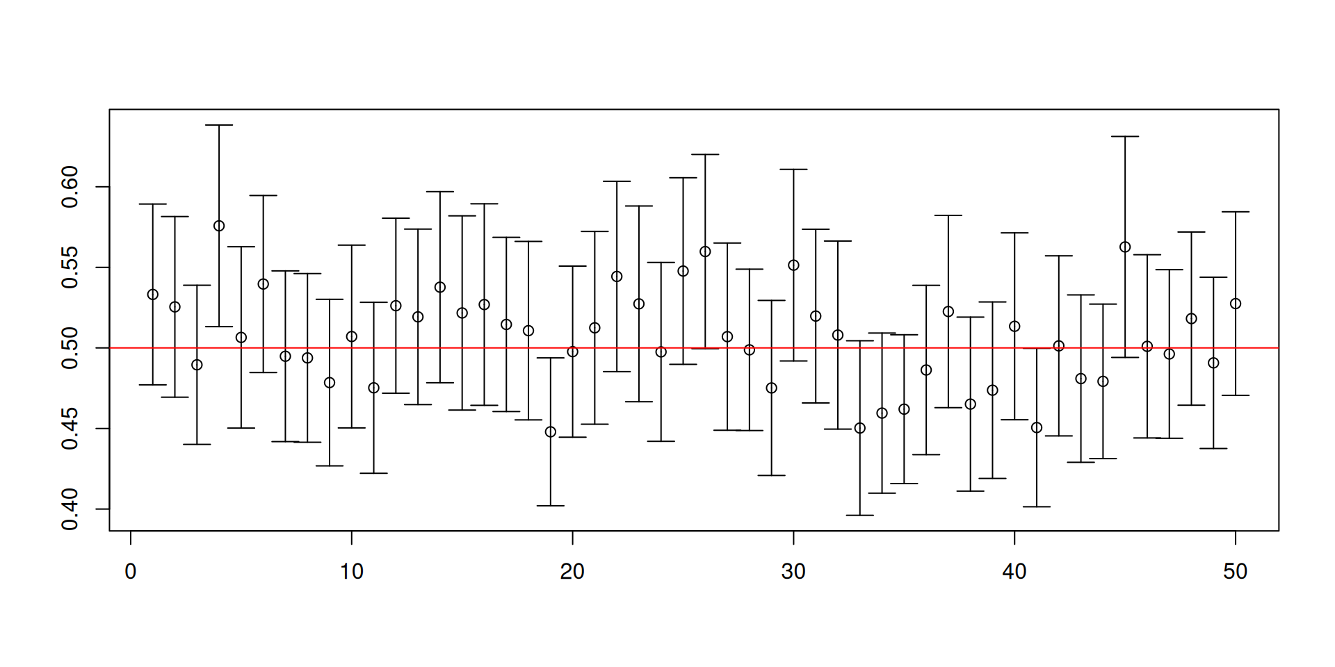
[1] 0.949[1] 0.0214 0.0296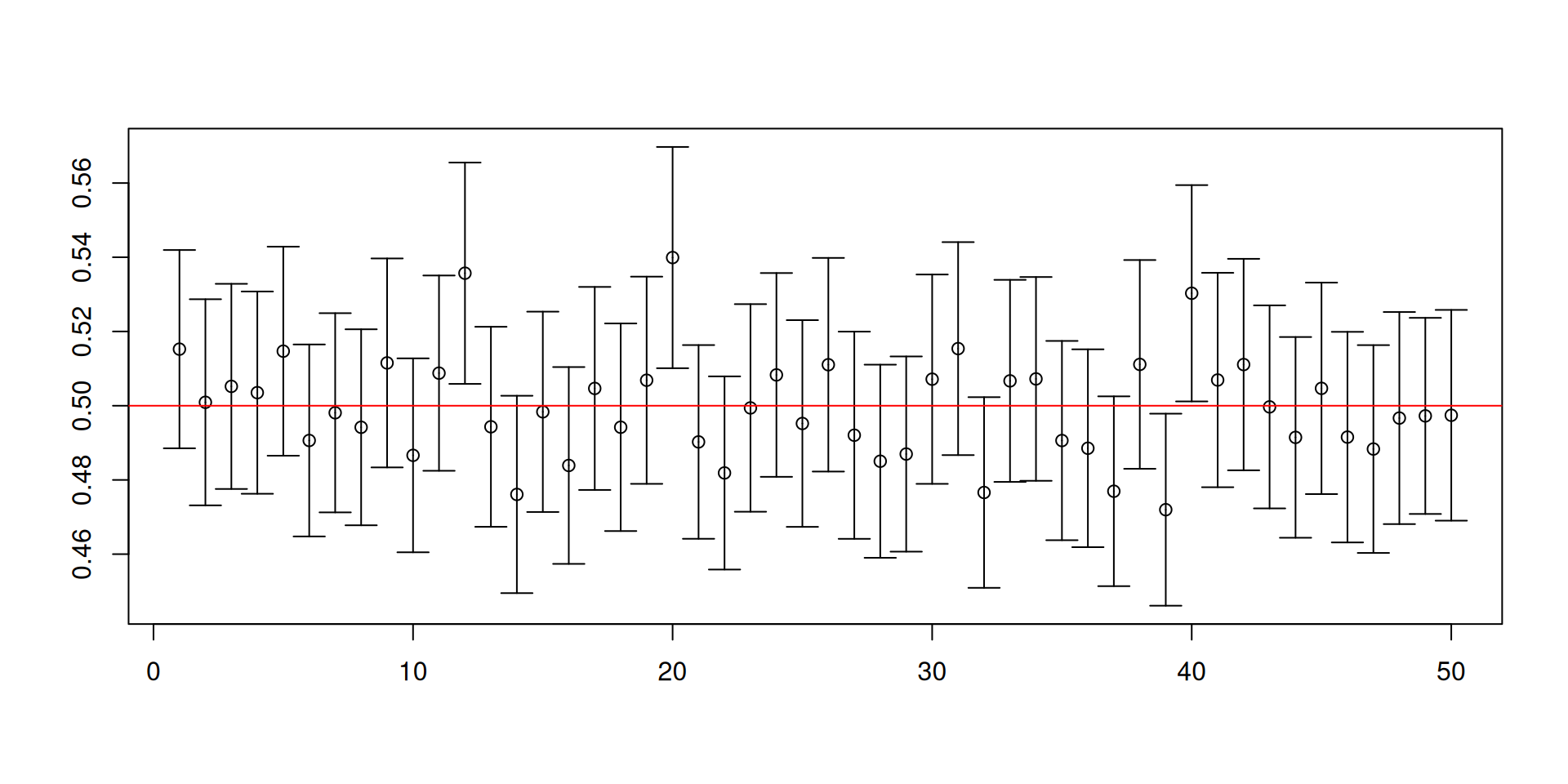
[1] 0.9494[1] 0.0238 0.0268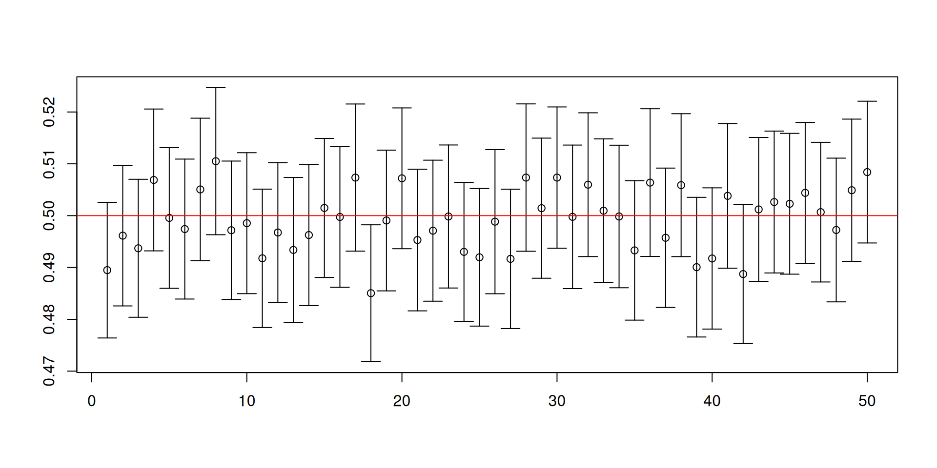
[1] 0.9492[1] 0.0248 0.0260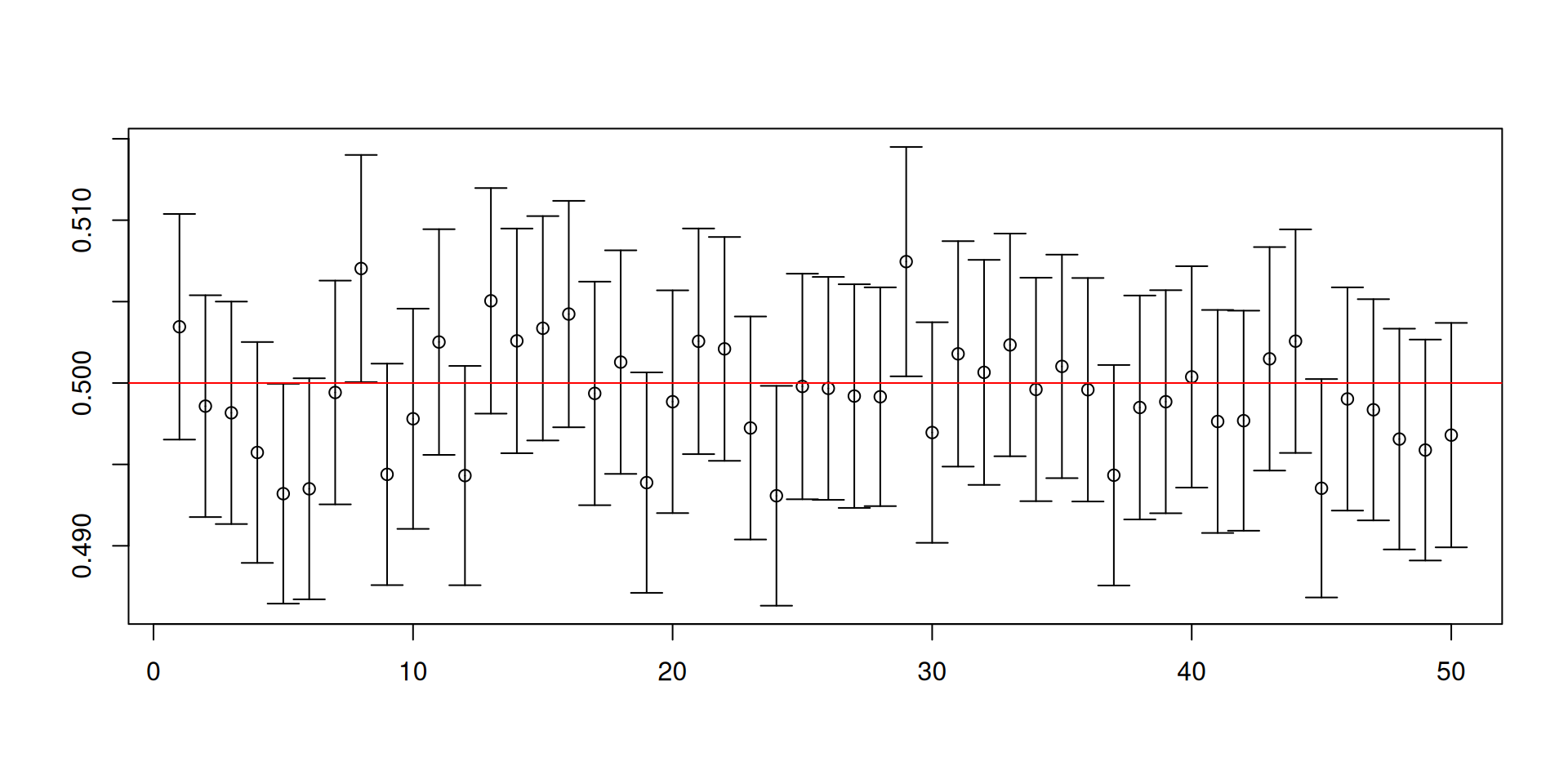
Warnings about confidence intervals
- The (procedure for constructing) confidence intervals has randomness while the unknown parameter is fixed!
- Furthermore, a confidence set is NOT a probability statement about the unknown parameter.
- You will NEVER know if the confidence set you have constructed for the ONE sample that you have actually contains the true value of the unknown parameter!
- It is the procedure that has the desired coverage properties.
Example: Testing hypotheses
Suppose a senator introduces a bill to simplify the tax code.
- The senator claims that his bill is revenue-neutral. This means that tax revenues will stay the same.
- Suppose the Treasury Department will evaluate the senator’s claim. The Treasury Department has more than a million representative set of tax returns.
We could have computed the difference between the tax obtained under the simplified tax code and the tax under the old tax code for all returns.
- The employee claims that the difference should be negative. Simplified tax code will bring in less revenues.
- The senator claims that the difference should be zero. Simplified tax code is revenue neutral.
But it is extremely time consuming to calculate this difference using all tax returns.
- An employee from the Treasury Department chooses a random sample of 100 tax returns from this tax file.
- The employee will then recompute the taxes to be paid under the simplified tax code and compare it with the taxes paid under the old tax code.
- He calculates the difference.
The employee finds that the sample average of the differences obtained from the 100 tax files was \(-219\) dollars and that the sample standard deviation of the differences is \(752\) dollars.
- The senator believes that it was only by chance that any difference would be negative.
- For example, the random sampling mechanism drew too many big negative numbers!
- The employee believes that it could not possibly be explained by chance.
So how do we evaluate both claims?
The framework for testing hypotheses
- Let \(X_i\) be the difference between the taxes obtained for the \(i\)th tax return.
- So, we have \(X_1,\ldots, X_{100}\) which are IID random variables having a common distribution.
- The target is the population mean of that distribution. Denote it by \(\mu\).
- The senator claims that \(\mu=0\) (actually \(\mu\geq 0\)). This is the null hypothesis.
- The employee claims that \(\mu <0\). This is the alternative hypothesis.
- But we do not observe \(\mu\). We only get to observe \(\overline{X}\).
- Although we get to observe \(\overline{X}\), it is subject to sampling variation.
- If the null were true, what would be typical values for \(\overline{X}\)?
Under the null and IID conditions, we know that the sampling distribution of \(\overline{X}\) is centered at 0, give or take, a standard error.
Suppose the employee finds that the sample average of the differences obtained from the 100 tax files was \(-219\) dollars and that the sample standard deviation of the differences is \(752\) dollars.
The observed sample mean is \(-219\) and the computed standard error is \(75.2\).
If the null were true, what is \(\mathbb{P}\left(\overline{X}<-219\right)\)?
By the CLT, we have the following approximation: \[ \begin{eqnarray*} \mathbb{P}\left(\overline{X} < -219\bigg\vert H_0\ \mathrm{is\ true}\right) &=& \mathbb{P}\left(\frac{\overline{X}-\mu}{s/\sqrt{100}} < \frac{-219-\mu}{s/\sqrt{100}}\bigg\vert H_0\ \mathrm{is\ true}\right) \\ &\approx & \mathbb{P}\left(Z< \frac{-219-\mu}{s/\sqrt{100}}\bigg\vert H_0\ \mathrm{is\ true}\right) \end{eqnarray*} \] where \(Z\sim N\left(0,1\right)\).
- Since the null (\(\mu=0\)) is assumed to be true, we have
\[ \mathbb{P}\left(Z< \frac{-219}{752/\sqrt{100}}\bigg\vert H_0\ \mathrm{is\ true}\right)\approx 0.0018 \]
What you computed is called a left-tailed \(p\)-value.
You now have to decide whether this \(p\)-value is compatible or incompatible with the null (leading to non-rejection or rejection of the null).
This decision depends on the truth of the null, which you will never know!
The null hypothesis could be true or false.
The decision you make given the data could be correct or incorrect.
In the end, you make two types of errors.
- Type I error: Reject the null when in fact it is true.
- Type II error: Do not reject the null when in fact it is false.
Suppose you decide to reject the null when \(\overline{X} \leq -219\). Then the probability of committing a Type I error is actually given by the previously calculated \(p\)-value.
You could have used different decision rules. For examples:
- Reject the null when \(\overline{X} \leq -50\). Then the probability of committing a Type I error is \(0.2531\).
- Reject the null when \(\overline{X} \leq -300\). Then the probability of committing a Type I error is \(3.31\times 10^{-5}\).
Notice that the null was assumed to be true in the calculations.
Notice that you may have to determine how much you are willing to risk making Type I errors.
There are two options:
- We could simply report the \(p\)-value and leave the decision to reject or not reject the null to someone else.
- Or, we accept that there are so many possible decision rules, therefore, we have to design a decision rule which is “well-calibrated”.
What do I mean by “well-calibrated”?
Usually we will have to set a significance level. The significance level \(\alpha\in (0,1)\) is the largest acceptable probability of committing a Type I error.
So, in our example, we want to find \(a\) such that the decision rule “Reject the null when \(\overline{X} \leq a\)” will have the probability of committing a Type I error about \(\alpha\).
Another possible decision rule is “Reject the null when the \(p\)-value is less than \(\alpha\)”.
- Let us “reverse-engineer” our existing calculations:
\[ \begin{eqnarray*} \alpha &=& \mathbb{P}\left(Z< c \mid H_0\ \mathrm{is\ true}\right) \\ & \approx & \mathbb{P}\left(\frac{\overline{X}-\mu}{s/\sqrt{100}} < c \bigg\vert H_0\ \mathrm{is\ true}\right) \\ &=& \mathbb{P}\left(\overline{X}< \mu+c\frac{s}{\sqrt{100}} \bigg\vert H_0\ \mathrm{is\ true}\right) \\ &=& \mathbb{P}\left(\overline{X}< c\frac{s}{\sqrt{100}} \bigg\vert H_0\ \mathrm{is\ true}\right) \end{eqnarray*} \]
The algorithm using the decision rule:
\(H_{0}:\;\mu=0\) and \(H_{1}:\;\mu<0\)
Set \(\alpha=0.05\).
Note that \(c=-1.65\).
We reject the null when \(\overline{X} < -1.65\times \frac{752}{\sqrt{100}}=-124.08\).
Decision: Since the observed value of \(\overline{X}\) is \(-219\), we reject \(H_{0}\) at the 5% level.
If the senator’s tax bill were revenue-neutral, then the observed 219 dollar reduction of tax revenues cannot be explained by chance alone.
Why would these decision rules be “well-calibrated”?
Let \(X_1,\ldots, X_n\) be IID random variables with an exponential distribution with rate parameter equal to 2.
Let us look at a test of hypothesis where \(H_0:\ \ \mu=1/2\) against \(H_1:\ \ \mu < 1/2\).
Set \(\alpha=0.05\).
Consider the decision rule: “Reject null when \(\overline{X} <1/2-1.65\times \sqrt{1/4}/\sqrt{n}\).
- This decision rule can be thought of as a “recipe” too. We can evaluate how often this rule makes errors. In particular, we focus on the relative frequency of Type I error.
test <- function(n)
{
  data <- rexp(n, 2)
  return(mean(data) < 1/2 + qnorm(0.05) * sqrt(1/4)/sqrt(n))
}
results <- replicate(10^4, sapply(c(5, 20, 80, 320, 1280), test))
apply(results, 1, mean)
[1] 0.0112 0.0295 0.0402 0.0461 0.0488- Notice what is happening to the relative frequency of Type I error.
Is there a relation to \(p\)-values?
- From the previous calculations in the tax example, you already found that \(\mathrm{P}\left(\overline{X}< -124.08 \vert H_0\ \mathrm{is\ true}\right) \approx \alpha\).
- You also found from the \(p\)-value calculation that \(\mathrm{P}\left(\overline{X}< -219\vert H_0\ \mathrm{is\ true}\right) \approx 0.0018\).
- So, if we decide to reject the null on the basis of the \(p\)-value, you would have to reject the null whenever the \(p\)-value is less than or equal to \(\alpha\).
Another simulation to show that \(p\)-value rule is well calibrated
test <- function(n)
{
  data <- rexp(n, 2)
  test.stat <- (mean(data)-1/2)/(sqrt(1/4)/sqrt(n))
  return(pnorm(test.stat) < 0.05)
}
results <- replicate(10^4, sapply(c(5, 20, 80, 320, 1280), test))
apply(results, 1, mean)
[1] 0.0115 0.0330 0.0418 0.0452 0.0508- Notice what is happening to the relative frequency of Type I error.
What do you know so far
Testing hypotheses require the following elements BEFORE seeing the data:
- Form the null and alternative hypotheses.
- Set the significance level \(\alpha\).
- Form a decision rule which is well-calibrated. This decision rule requires you to think of test statistics.
AFTER seeing the data, you could apply your decision rule. Make a conclusion that is readable to broad audiences.
Note that the structure of a hypothesis test forces you to think of the statistical model behind the way the data are generated.
Setting the significance level forces you to think of the Type I error.
Forming the decision rule forces you to think about the test statistic and its distribution under the null.
These are all done BEFORE seeing the data. It is easy to see why the framework is subject to manipulation, confusion, and misunderstanding.
Moving on to more complicated models
- You now have the basics of key inference tasks, at least when conducting inference about the population mean.
- The common model that enables us to carry out these tasks is the signal plus noise model.
- In the next set of slides, I recap the signal plus noise model, which you have seen before.
Carrying out these inference tasks without a model is absurd. Why?
- Because there is a thought experiment involving drawing repeated samples.
- Because we use a sampling distribution, which is constructed hypothetically.
I then extend to different versions of linear regression models, which nests the signal plus noise model.
For every model, I point out the parameters of interest and the key statistical results for the procedures used to estimate these parameters.
Signal plus noise model
- Let \(X_1, \ldots, X_n\) be IID random variables where \[X_t=\mu+\varepsilon_t\]
- The \(\varepsilon_t\)’s are IID random variables with \(\mathbb{E}\left(\varepsilon_t\right)=0\) and \(\mathsf{Var}\left(\varepsilon_t\right)=\sigma^2\).
- \(\mu\) is a population parameter of interest we want to learn about.
- The sample mean \(\overline{X}\) is usually used to estimate \(\mu\).
Recall that when \(n\) is fixed, we have \(\mathbb{E}\left(\overline{X}\right)= \mu\) and \(\mathsf{Var}\left(\overline{X}\right) = \sigma^2/n\).
When \(n\to\infty\), we have:
\[\begin{eqnarray*} \overline{X} &\overset{p}{\to}& \mu\\ \frac{\overline{X}-\mu}{\sigma/\sqrt{n}} &\overset{d}{\to}& N(0,1) \end{eqnarray*}\]
The CLT result is sometimes written as \[\sqrt{n}\left(\overline{X}-\mu\right)\overset{d}{\to} N\left(0,\sigma^2\right)\] Here \(\sigma^2\) is called the asymptotic variance of \(\sqrt{n}\left(\overline{X}-\mu\right)\).
We need a consistent plug-in for the asymptotic variance. Here we use the sample variance or if you wish the square of the sample standard deviation.
Fixed-\(\mathbf{X}\) linear regression model
A1 Let \(X_t^\prime=(1, X_{1t}, X_{2t}, \ldots X_{kt})\) be the regressors. The matrix \(\mathbf{X}\) does NOT vary across repeated samples and \(\mathbf{X}^\prime \mathbf{X}\) is invertible.
Further assume that
- A2 For all \(t\), we have \(Y_t=X_t^\prime\beta+\varepsilon_t\)
- A3 \(\varepsilon_t\)’s satisfy \(\mathbb{E}\left(\varepsilon_t\right)=0\) for all \(t\).
- A4 \(\varepsilon_t\)’s satisfy \(\mathsf{Var}\left(\varepsilon_t\right)=\sigma^2\) for all \(t\) and \(\mathsf{Cov}\left(\varepsilon_t,\varepsilon_s\right)\) for all \(t\neq s\).
\(\mathsf{Var}\left(\varepsilon_t\right)=\sigma^2\) for all \(t\) is sometimes called the homoscedasticity assumption.
\(\mathsf{Cov}\left(\varepsilon_t,\varepsilon_s\right)\) for all \(t\neq s\) is sometimes called the no serial correlation or no spatial correlation assumption.
Sometimes A3, A4, and A5 are replaced by a stronger version saying \(\varepsilon_t\)’s are zero mean IID random variables.
The signal plus noise model is a special case of this model. Just set \(X_t^\prime=1\).
\(\beta\) is a population parameter of interest we want to learn about.
To estimate \(\beta\), we use the OLS estimator \(\widehat{\beta}\).
When \(n\) is fixed, it can be shown that:
- Under A1 to A3, we have \(\mathbb{E}\left(\widehat{\beta}\right) = \beta\).
- Under A1 to A4, we have \(\mathsf{Var}\left(\widehat{\beta}\right)=\sigma^2 \left(\mathbf{X}^\prime \mathbf{X}\right)^{-1}\).
There are results when \(n\to\infty\), but I skip them.
Correctly specified linear regression model, version 1
- A1 \(\{\left(Y_t, X_t^\prime\right)\}_{t=1}^n\) are observable random vectors, where \(\mathbf{X}^\prime \mathbf{X}\) is invertible.
- A2 For all \(t\), we have \(Y_t=X_t^\prime\beta+\varepsilon_t\).
- A3 \(\varepsilon_t\)’s satisfy \(\mathbb{E}\left(\varepsilon_t|X_1^\prime,X_2^\prime, \ldots, X_n^\prime\right)=0\) for all \(t\).
- A4 \(\varepsilon_t\)’s satisfy \(\mathsf{Var}\left(\varepsilon_t|X_1^\prime,X_2^\prime, \ldots, X_n^\prime\right)=\sigma^2\) for all \(t\).
- A5 \(\varepsilon_t\)’s satisfy \(\mathsf{Cov}\left(\varepsilon_t,\varepsilon_s|X_1^\prime,X_2^\prime, \ldots, X_n^\prime\right)=0\) for all \(t\neq s\).
\(\beta\) is a population parameter of interest we want to learn about.
To estimate \(\beta\), we use the OLS estimator \(\widehat{\beta}\).
When \(n\) is fixed, it can be shown that:
- Under A1, A2, and A3, \(\mathbb{E}\left(\widehat{\beta}|\mathbf{X}\right) = \beta\).
- Under A1, A2 to A5, \(\mathsf{Var}\left(\widehat{\beta}|\mathbf{X}\right)=\sigma^2 \left(\mathbf{X}^\prime \mathbf{X}\right)^{-1}\).
There are results when \(n\to\infty\), but I skip them.
Correctly specified linear regression model, version 2
- A1 \(\{\left(Y_t, X_t^\prime\right)\}_{t=1}^n\) are observable IID random vectors, where \(\mathbf{X}^\prime \mathbf{X}\) is invertible.
- A2 For all \(t\), we have \(Y_t=X_t^\prime\beta+\varepsilon_t\).
- A3 \(\varepsilon_t\)’s satisfy \(\mathbb{E}\left(\varepsilon_t|X_t^\prime\right)=0\) for all \(t\).
- A4 \(\varepsilon_t\)’s satisfy \(\mathsf{Var}\left(\varepsilon_t|X_t^\prime\right)=\sigma^2\) for all \(t\).
A1-1 Replace “\(\mathbf{X}^\prime \mathbf{X}\) is invertible” in A1 with “\(Q=\mathbb{E}\left(X_tX_t^\prime\right)\) is invertible”.
\(\beta\) is a population parameter of interest we want to learn about.
To estimate \(\beta\), we use the OLS estimator \(\widehat{\beta}\).
When \(n\) is fixed, it can be shown that:
- Under A1, A2, and A3, \(\mathbb{E}\left(\widehat{\beta}|\mathbf{X}\right) = \beta\).
- Under A1, A2 to A4, \(\mathsf{Var}\left(\widehat{\beta}|\mathbf{X}\right)=\sigma^2 \left(\mathbf{X}^\prime \mathbf{X}\right)^{-1}\).
When \(n\to\infty\), it can be shown that:
- Under A1-1, A2, and A3, \(\widehat{\beta} \overset{p}{\to} \beta\).
- Under A1-1, A2, A3, and finite second moments,
\[\sqrt{n}\left(\widehat{\beta}-\beta\right) \overset{d}{\rightarrow} N\left(0,\mathbb{E}\left(X_{t}X_{t}^{\prime}\right)^{-1}\mathbb{E}\left(X_{t}X_{t}^{\prime}\varepsilon_t^2\right)\mathbb{E}\left(X_{t}X_{t}^{\prime}\right)^{-1}\right)\]
Assumption-lean linear regression model
- A1-1 \(\{\left(Y_t, X_t^\prime\right)\}_{t=1}^n\) are observable IID random vectors, where \(\mathbb{E}\left(X_tX_t^\prime\right)\) is invertible.
- A2 For all \(t\), we have \(Y_t=X_t^\prime\beta+\varepsilon_t\).
- A3 \(\varepsilon_t\)’s satisfy \(\mathbb{E}\left(\varepsilon_t\right)=0\) and \(\mathbb{E}\left(X_t\varepsilon_t\right)=0\) for all \(t\).
- With this set of assumptions, the \(\beta\) in A2 is really \(\beta^*\), the coefficients of the best linear predictor of \(Y\) given the \(X\)’s.
- \(\beta^*\) is a population parameter of interest we want to learn about.
- To estimate \(\beta^*\), we use the OLS estimator \(\widehat{\beta}\).
- We CANNOT establish unbiasedness for \(\beta^*\) under the assumption-lean linear regression model.
- We can only asymptotically justify the use of the OLS estimator.
When \(n\to\infty\), it can be shown that:
- Under A1-1, A2, and A3, \(\widehat{\beta} \overset{p}{\to} \beta^*\).
- Under A1-1, A2, A3, and finite second moments,
\[\sqrt{n}\left(\widehat{\beta}-\beta^*\right) \overset{d}{\rightarrow} N\left(0,\mathbb{E}\left(X_{t}X_{t}^{\prime}\right)^{-1}\mathbb{E}\left(X_{t}X_{t}^{\prime}\varepsilon_t^2\right)\mathbb{E}\left(X_{t}X_{t}^{\prime}\right)^{-1}\right)\]
Consistent estimation of \(\mathsf{Avar}\left(\sqrt{n}\left(\widehat{\beta}-\beta\right)\right)\)
Typically, you would need an additional assumption of finite fourth moments to be able to consistently estimate \[\mathsf{Avar}\left(\sqrt{n}\left(\widehat{\beta}-\beta\right)\right)=\mathbb{E}\left(X_{t}X_{t}^{\prime}\right)^{-1}\mathbb{E}\left(X_{t}X_{t}^{\prime}\varepsilon_t^2\right)\mathbb{E}\left(X_{t}X_{t}^{\prime}\right)^{-1}\]
This is the heteroscedasticity-consistent (HC) version of the asymptotic variance.
Later, we will show that under A4, we can simplify this to \[\mathsf{Avar}\left(\sqrt{n}\left(\widehat{\beta}-\beta\right)\right)=\sigma^2\mathbb{E}\left(X_{t}X_{t}^{\prime}\right)^{-1}\]
This is the homoscedasticity-only (HO) version of the asymptotic variance. This is the default in
baseR.You will need non-
basepackages to compute other types of asymptotic variances.
The components of \(\mathsf{Avar}\left(\sqrt{n}\left(\widehat{\beta}-\beta\right)\right)\) rely on population quantities. For the HC version, we need:
- To consistently estimate the “bread” \(Q=\mathbb{E}\left(X_{t}X_{t}^{\prime}\right)\): This is straightforward.
- To consistently estimate the “meat” \[\mathsf{Avar}\left(\dfrac{1}{\sqrt{n}}{\displaystyle \sum_{t=1}^{n}}X_{t}\varepsilon_{t}\right)=\lim_{n\rightarrow\infty}\mathsf{Var}\left(\dfrac{1}{\sqrt{n}}{\displaystyle \sum_{t=1}^{n}}X_{t}\varepsilon_{t}\right).\]
- Consistently estimating the “meat” depends on assumptions regarding the sequence of observations \(\left\{\left(X_t, \varepsilon_t\right)\right\}_{t=1}^n\).
- Under Version 2 of the correctly specified linear regression model with A1-1, A2, and A3 or under the assumption-lean linear regression model, \[\mathsf{Avar}\left(\dfrac{1}{\sqrt{n}}{\displaystyle \sum_{t=1}^{n}}X_{t}\varepsilon_{t}\right)= \mathbb{E}\left(X_tX_t^\prime \varepsilon_t^2\right)\]
It can be shown that a consistent estimator of \(\mathsf{Avar}\left(\sqrt{n}\left(\widehat{\beta}-\beta\right)\right)\) is of the following form: \[\left(\frac{1}{n}\sum_{t=1}^n X_tX_t^\prime\right)^{-1}\left(\frac{1}{n}\sum_{t=1}^n X_tX_t^\prime e_t^2\right)\left(\frac{1}{n}\sum_{t=1}^n X_tX_t^\prime\right)^{-1}\] where \(e_t\) is the OLS residual.
We denote this as \(\widehat{\mathsf{Avar}}\left(\sqrt{n}\left(\widehat{\beta}-\beta\right)\right)\).
The variance-covariance matrix (or
vcovin R) which you need and would be the source of your standard errors is computed as \[\frac{1}{n} \cdot \widehat{\mathsf{Avar}}\left(\sqrt{n}\left(\widehat{\beta}-\beta\right)\right)\]Taking the square root of the main diagonal of the preceding matrix gives you the standard errors. The \(j\)th entry of that main diagonal is the standard error for \(\widehat{\beta}_j\).
Special case: One coefficient of interest
It can be shown that \[\sqrt{n}\left(\widehat{\beta}_j-\beta^*_j \right)\overset{d}{\rightarrow}N\left(0,\dfrac{\mathbb{E}\left(v_{t}^{2}\varepsilon_{t}^{2}\right)}{\left[\mathbb{E}\left(v_{t}^{2}\right)\right]^{2}}\right),\] where \(v_t\) is the error from the best linear prediction of \(X_j\) given \(X_{-j}\).
\(X_{-j}\) is really all the other \(X\)’s aside from the \(j\)th regressor.
This notation should remind you of FWL.
Special case: Correct specification plus conditional homoscedasticity
- Under Version 2 of the correctly specified linear regression model and further assuming A4, it is possible to show that \[\begin{eqnarray*}\mathsf{Var}\left(X_{t}\varepsilon_{t}\right) &=&\mathbb{E}\left(X_{t}X_{t}^{\prime}\varepsilon_{t}^{2}\right) \\ &=&\mathbb{E}\left(\mathbb{E}\left(X_{t}X_{t}^{\prime}\varepsilon_{t}^{2}|X_{t}\right)\right) \\ &=&\mathbb{E}\left(X_{t}X_{t}^{\prime}\mathbb{E}\left(\varepsilon_{t}^{2}|X_{t}\right)\right)=\sigma^{2}\mathbb{E}\left(X_{t}X_{t}^{\prime}\right)\end{eqnarray*}\]
It makes sense to impose correct specification in the conditional homoscedasticity case, because, \[\begin{eqnarray*}\sigma^{2} &=&\mathsf{Var}\left(\varepsilon_{t}|X_{t}\right) \\ &=&\mathbb{E}\left(\varepsilon_{t}^{2}|X_{t}\right)-\left(\mathbb{E}\left(\varepsilon_{t}|X_{t}\right)\right)^2=\mathbb{E}\left(\varepsilon_{t}^{2}|X_{t}\right)\end{eqnarray*}\]
Therefore, we have \[\begin{eqnarray*}\mathsf{Avar}\left(\sqrt{n}\left(\widehat{\beta}-\beta\right)\right) &=& \mathbb{E}\left(X_{t}X_{t}^{\prime}\right)^{-1}\sigma^2\mathbb{E}\left(X_{t}X_{t}^{\prime}\right)\mathbb{E}\left(X_{t}X_{t}^{\prime}\right)^{-1} \\ &=&\sigma^{2}\mathbb{E}\left(X_{t}X_{t}^{\prime}\right)^{-1}\end{eqnarray*}\]
Special case: One coefficient of interest again
- Stay within Version 2 of the correctly specified linear regression model and assume A4.
- It can be shown that \[\mathsf{Avar}\left(\sqrt{n}\left(\widehat{\beta}_j-\beta_{j}\right)\right)=\dfrac{\sigma^{2}}{\mathbb{E}\left(v_{t}^{2}\right)}=\dfrac{\sigma^{2}}{\left(1-R_{j,-j}^{2}\right)\mathsf{Var}\left(X_{tj}\right)}\]
The components are as follows:
- \(R_{j,-j}^{2}\) is the population R-squared from the best linear prediction of \(X_{j}\) using \(X_{-j}\)
- \(\mathsf{Var}\left(X_{tj}\right)\) is the population variance of \(X_{tj}\).
The result tells you what makes asymptotic variances large. You can trace to three sources.
- Noise from error from best prediction
- Spread of the \(j\)th regressor
- Extent of linear relationship between \(X_j\) and \(X_{-j}\)
Detour: Relationship to imperfect multicollinearity
The result in the previous two slides is an important special case and has been a source of utter confusion and mess!
The result under conditional homoscedasticity is where all the “scariness” of imperfect multicollinearity comes from.
Note that as \(R_{j,-j}^{2}\to 1\), \(\mathsf{Avar}\left(\sqrt{n}\left(\widehat{\beta}_{j}-\beta_{j}\right)\right)\to\infty\).
Therefore, if \(X_{j}\) is almost a linear function of \(X_{-j}\), then it is not surprising that you become much more uncertain about \(\widehat{\beta}_{j}\).
There is no “testing” for the presence of imperfect multicollinearity as it is always present, especially when dealing with observational data.
Some have proposed “rules of thumb” to “diagnose” how severe things could be, but these are developed under the assumption of conditional homoscedasticity.
A better use of your time would be to understand why there is imperfect multicollinearity in your application.
SEs for linear functions of the estimated parameters
Let \(R\) be a nonstochastic \(J\times K\) matrix with rank \(J\leq K\).
- This means that \(R\) does not have any “redundancies”.
Provided that \(\sqrt{n}\left(\widehat{\beta}-\beta\right)\overset{d}{\to}N\left(0,\Omega\right)\), then we have \[\sqrt{n}\left(R\widehat{\beta}-R\beta\right) \overset{d}{\to} N\left(0,R\Omega R^{\prime}\right).\]
SEs for nonlinear functions of the estimated parameters
Here we are interested in a nonlinear function \(R\left(\beta\right)\) where \(\dfrac{\partial R\left(\beta\right)}{\partial\beta}\) is a nonstochastic \(J\times K\) matrix with rank \(J\leq K\).
Provided that \(\sqrt{n}\left(\widehat{\beta}-\beta\right)\overset{d}{\to}N\left(0,\Omega\right)\), then \[\sqrt{n}\left(R\left(\widehat{\beta}\right)-R\left(\beta\right)\right) \overset{d}{\to} N\left(0,\dfrac{\partial R\left(\beta\right)}{\partial\beta}\Omega\left(\dfrac{\partial R\left(\beta\right)}{\partial\beta}\right)^{\prime}\right).\]
Confidence intervals and hypothesis tests
The earlier distributional results imply that the statistic \[\left[\sqrt{n}\left(R\widehat{\beta}-R\beta\right)\right]^{\prime}\left(R\Omega R^{\prime}\right)^{-1}\sqrt{n}\left(R\widehat{\beta}-R\beta^{*}\right)\overset{d}{\to}\chi_{J}^{2}\]
Under the null \(R\beta=q\) for linear hypotheses, we have \[\left[\sqrt{n}\left(R\widehat{\beta}-q\right)\right]^{\prime}\left(R\Omega R^{\prime}\right)^{-1}\sqrt{n}\left(R\widehat{\beta}-q\right)\overset{d}{\to}\chi_{J}^{2}\]
- A similar set of results can be derived for nonlinear hypotheses.
- In a lot of applied work I have seen, \(J\) would typically be equal to 1. Of course, there are exceptions.
- There is a new distribution in the result. It is called the chi-squared distribution with \(J\) degrees of freedom, denoted by \(\chi^2_J\).
- In finite samples, it can be approximated by \(J\) times an \(F\) distribution with \(J\) numerator degrees of freedom and \(n-\left(k+1\right)\) denominator degrees of freedom, denoted by \(J\cdot F_{J,n-\left(k+1\right)}\).
- This follows from \(J\cdot F_{J,n-\left(k+1\right)}\overset{d}{\to} \chi^2_J\), as \(n\to\infty\).
- We now work on a special case that comes by default in
baseR. - Assume conditional homoscedasticity A4 and assume that we are testing linear hypotheses that \(R\beta=q\).
- Recall that \[\mathsf{Avar}\left(\sqrt{n}\left(\widehat{\beta}-\beta\right)\right) =\sigma^{2}\mathbb{E}\left(X_{t}X_{t}^{\prime}\right)^{-1}\]
- \(s^2=e^\prime e/\left(n-(k+1)\right)\) or \(s^2=e^\prime e/n\) are consistent estimators of \(\sigma^2\).
- The test statistic may be simplified into an even more intuitive form, but is limited by its assumptions.
\[\begin{eqnarray*} && \left[\sqrt{n}\left(R\widehat{\beta}-q\right)\right]^{\prime}\left(Rs^2 \widehat{Q}^{-1} R^{\prime}\right)^{-1}\sqrt{n}\left(R\widehat{\beta}-q\right) \\&=& \dfrac{\left(R\widehat{\beta}-q\right)^\prime \left(R \left(\mathbf{X}^\prime\mathbf{X}\right)^{-1} R^{\prime}\right)^{-1}\left(R\widehat{\beta}-q\right)}{e^\prime e/\left(n-(k+1)\right)} \\ &=& \dfrac{\widetilde{e}^{\prime}\widetilde{e}-e^{\prime}e}{e^\prime e/\left(n-(k+1)\right)} = J \cdot \dfrac{\left(\widetilde{e}^{\prime}\widetilde{e}-e^{\prime}e\right)/J}{e^\prime e/\left(n-(k+1)\right)} \end{eqnarray*}\]
- \(e^\prime e\) is the sum of squared residuals (the minimized least squares objective function) of the unrestricted model.
- \(\widetilde{e}^{\prime}\widetilde{e}\) is the sum of squared residuals of the restricted model.
- So, intuitively the test statistic is comparing fit of the unrestricted and restricted models!
- The \(F\)-statistic found
summary()after saving anlm()object is actually computed using: \[\dfrac{\left(\widetilde{e}^{\prime}\widetilde{e}-e^{\prime}e\right)/J}{e^\prime e/\left(n-(k+1)\right)}\]
Illustrating Hamermesh and Parker (2005)
Recall Exercise Set 5.
The authors use weighted least squares where the weight variable is the number of students completing the evaluation forms in each class.
options(digits = 2)
ratings <- read.csv("ProfEvaltnsBeautyPublic.csv")
tab3.all <- lm(courseevaluation ~ btystdave + female + minority + nonenglish + tenuretrack + lower + onecredit, weights = didevaluation, data = ratings)
coef(tab3.all)
(Intercept) btystdave female minority nonenglish tenuretrack
4.247 0.275 -0.239 -0.249 -0.253 -0.136
lower onecredit
-0.046 0.687 - Next, I present three sets of estimates of the variance-covariance matrix, which is really \(\widehat{\mathsf{Avar}}\left(\sqrt{n}\left(\widehat{\beta}-\beta\right)\right)/n\).
- This is more in line with the setup of the Version 2 of the correctly specified linear regression model with A4 imposed.
            (Intercept) btystdave   female minority nonenglish tenuretrack
(Intercept)     0.00427   2.1e-04 -1.2e-03  0.00047   -3.0e-04    -3.5e-03
btystdave       0.00021   7.6e-04  3.3e-06 -0.00011    7.8e-05    -2.2e-04
female         -0.00117   3.3e-06  2.1e-03 -0.00097    2.0e-04     4.5e-04
minority        0.00047  -1.1e-04 -9.7e-04  0.00640   -3.2e-03    -5.3e-04
nonenglish     -0.00030   7.8e-05  2.0e-04 -0.00317    1.4e-02    -4.1e-04
tenuretrack    -0.00351  -2.2e-04  4.5e-04 -0.00053   -4.1e-04     3.9e-03
lower          -0.00096  -1.1e-04  2.3e-04 -0.00021    7.9e-04     7.7e-05
onecredit      -0.00202   3.2e-04  6.2e-04 -0.00300    4.8e-04     2.3e-03
               lower onecredit
(Intercept) -9.6e-04  -0.00202
btystdave   -1.1e-04   0.00032
female       2.3e-04   0.00062
minority    -2.1e-04  -0.00300
nonenglish   7.9e-04   0.00048
tenuretrack  7.7e-05   0.00228
lower        1.9e-03  -0.00097
onecredit -9.7e-04 0.01873- This is more in line with the setup of the assumption-lean linear regression model.
            (Intercept) btystdave   female minority nonenglish tenuretrack
(Intercept)     0.00445   4.3e-04 -0.00178  3.9e-04    0.00006    -0.00331
btystdave       0.00043   1.3e-03 -0.00046 -6.1e-05    0.00016    -0.00034
female         -0.00178  -4.6e-04  0.00345 -1.1e-03   -0.00039     0.00052
minority        0.00039  -6.1e-05 -0.00106  9.0e-03   -0.00363    -0.00065
nonenglish      0.00006   1.6e-04 -0.00039 -3.6e-03    0.01069    -0.00072
tenuretrack    -0.00331  -3.4e-04  0.00052 -6.5e-04   -0.00072     0.00385
lower          -0.00199  -5.9e-05  0.00057 -5.7e-04    0.00084     0.00089
onecredit      -0.00054   5.6e-04  0.00076 -4.7e-03    0.00072     0.00095
               lower onecredit
(Intercept) -2.0e-03  -0.00054
btystdave   -5.9e-05   0.00056
female       5.7e-04   0.00076
minority    -5.7e-04  -0.00468
nonenglish   8.4e-04   0.00072
tenuretrack  8.9e-04   0.00095
lower        3.9e-03  -0.00237
onecredit -2.4e-03 0.01447- The paper uses “… robust standard errors that account for the clustering of the observations (because we observe multiple classes for the overwhelming majority of instructors) …”
            (Intercept) btystdave   female minority nonenglish tenuretrack
(Intercept)     0.00958   0.00064 -0.00199  0.00081   -0.00092    -7.5e-03
btystdave       0.00064   0.00345 -0.00106 -0.00083    0.00006     2.8e-04
female         -0.00199  -0.00106  0.00725 -0.00238   -0.00013    -3.0e-04
minority        0.00081  -0.00083 -0.00238  0.01247   -0.00450    -1.7e-03
nonenglish     -0.00092   0.00006 -0.00013 -0.00450    0.01795    -6.0e-04
tenuretrack    -0.00754   0.00028 -0.00030 -0.00168   -0.00060     8.9e-03
lower          -0.00401   0.00061 -0.00152 -0.00169    0.00250     2.6e-03
onecredit       0.00055   0.00102  0.00159 -0.00209   -0.00209     6.5e-05
               lower onecredit
(Intercept) -0.00401   5.5e-04
btystdave    0.00061   1.0e-03
female      -0.00152   1.6e-03
minority    -0.00169  -2.1e-03
nonenglish   0.00250  -2.1e-03
tenuretrack  0.00261   6.5e-05
lower        0.01015  -6.0e-03
onecredit -0.00595 2.7e-02- Here we design a very rough table.
cbind("Coef" = coef(tab3.all), "Default SE" = sqrt(diag(vcov(tab3.all))), "HC SE" = sqrt(diag(vcovHC(tab3.all))), "Clustered SE" = sqrt(diag(vcovCL(tab3.all, cluster= ~ profnumber)))) Coef Default SE HC SE Clustered SE
(Intercept) 4.247 0.065 0.067 0.098
btystdave 0.275 0.028 0.036 0.059
female -0.239 0.046 0.059 0.085
minority -0.249 0.080 0.095 0.112
nonenglish -0.253 0.120 0.103 0.134
tenuretrack -0.136 0.062 0.062 0.094
lower -0.046 0.044 0.062 0.101
onecredit 0.687 0.137 0.120 0.166- In previous slides, we did not explicitly discuss clustered standard errors, but it does show up a lot in applied work. In your projects, you might also encounter this type of standard errors.
- Example: 95% large-sample confidence intervals for \(\beta_j\)
- Example: Testing \(\beta_j=0\)
coeftest(tab3.all, vcov = vcovCL(tab3.all, cluster = ~ profnumber), df = Inf) # Needs lmtest package
z test of coefficients:

            Estimate Std. Error z value Pr(>|z|)
(Intercept)   4.2474     0.0979   43.39  < 2e-16 ***
btystdave     0.2748     0.0587    4.68  2.9e-06 ***
female       -0.2390     0.0851   -2.81    0.005 **
minority     -0.2489     0.1117   -2.23    0.026 *
nonenglish   -0.2527     0.1340   -1.89    0.059 .
tenuretrack  -0.1359     0.0942   -1.44    0.149
lower        -0.0459     0.1007   -0.46    0.649
onecredit     0.6865     0.1655    4.15  3.4e-05 ***
---
Signif. codes: 0 '***' 0.001 '**' 0.01 '*' 0.05 '.' 0.1 ' ' 1- Example: Testing whether all population regression slopes are all equal to zero \(\beta_1=\beta_2=\cdots=\beta_7=0\):
library(car)
coefindex <- names(coef(tab3.all))
linearHypothesis(tab3.all, coefindex[-1], rhs = 0, test = "Chisq", vcov. = vcovCL(tab3.all, cluster = ~ profnumber))
Linear hypothesis test
Hypothesis:
btystdave = 0
female = 0
minority = 0
nonenglish = 0
tenuretrack = 0
lower = 0
onecredit = 0
Model 1: restricted model
Model 2: courseevaluation ~ btystdave + female + minority + nonenglish +
tenuretrack + lower + onecredit
Note: Coefficient covariance matrix supplied.
Res.Df Df Chisq Pr(>Chisq)
1 462
2 455 7 56.9 6.4e-10 ***
---
Signif. codes: 0 '***' 0.001 '**' 0.01 '*' 0.05 '.' 0.1 ' ' 1- Example: Testing whether all population regression slopes related to course type are all equal to zero \(\beta_6=\beta_7=0\):
linearHypothesis(tab3.all, c("lower", "onecredit"), rhs = 0, test = "Chisq", vcov. = vcovCL(tab3.all, cluster = ~ profnumber))Linear hypothesis test
Hypothesis:
lower = 0
onecredit = 0
Model 1: restricted model
Model 2: courseevaluation ~ btystdave + female + minority + nonenglish +
tenuretrack + lower + onecredit
Note: Coefficient covariance matrix supplied.
Res.Df Df Chisq Pr(>Chisq)
1 457
2 455 2 18.4 1e-04 ***
---
Signif. codes: 0 '***' 0.001 '**' 0.01 '*' 0.05 '.' 0.1 ' ' 1Introducing the bootstrap
- For averages, we can approximate probabilities involving averages using the central limit theorem. But this requires \(n\to\infty\) and requires that you are focusing on averages.
- As you recall, the CLT involves a standardized quantity. So, you need a standard error.
- You may encounter estimators which don’t involve just an average but functions of an average, or not even averages at all (minimum and median, for example).
The bootstrap principle
The bootstrap may be used to estimate bias, estimate standard errors, construct confidence intervals, and conduct hypothesis tests.
The idea is as follows.
- You have data on hand.
- There was a sampling mechanism which produced the data you have.
- But you do not know or you do not have full information about the mechanism which produced the data you have.
- So what do you do? You cannot use a Monte Carlo simulation (where we essentially knew everything).
- You sample from the data you have on hand. You are going to resample.
- We are NOT creating new data, unlike the artificial datasets generated by Monte Carlo.
- We have to resample in the same way that reflects the sampling mechanism which generated the data.
- Bottom line: we are not adding anything new, but we are injecting randomness into the problem so that we can get a sense of the sampling distribution.
The bootstrap principle for the sample mean
Here is one bootstrap principle for the sample mean which reflect IID conditions.
(Real world) Let \(x_1,\ldots,x_n\) be the data you actually have. Let \(\overline{x}\) be the actual sample mean.
(Bootstrap world) Let \(X_1^*, \ldots, X_n^*\) be a resample with replacement from \(x_1,\ldots,x_n\). Let \(\overline{X}^*\) be a bootstrapped sample mean.
(Bootstrap replicates) Collect an arbitrarily large \(B\) resamples of the bootstrapped sample mean, denoted by \(\overline{X}^*_{(1)}, \ldots, \overline{X}^*_{(B)}\).
(Bootstrap principle) Provided \(n\) is large, the bootstrap distribution of the \(\overline{X}^*-\overline{X}\) will be a good approximation to the sampling distribution of \(\overline{X}-\mu\).
There would be different bootstrap principles to approximate sampling distributions of the objects you are interested in. These principles have to be proven!
Three of the key versions of the bootstrap:
- Theoretical or exhaustive: Enumerate all possible resamples and construct the bootstrapped distribution of the estimator.
- Empirical or nonparametric bootstrap: Use the data you have, take them as fixed, and resample from them a large number of times.
- Parametric bootstrap: Fit a distribution which matches the data you have and draw resamples from that distribution.
The principle alone also does not tell you what kind of sample statistics may be bootstrapped. Be careful.
There are different tasks available for the bootstrap:
- Estimating the bias of a sample statistic
- Estimating the variance / standard error of a sample statistic
- Approximating probabilities: leads to confidence intervals and hypothesis testing
Let us study what the bootstrap is actually doing from the point of view of the theoretical or exhaustive bootstrap.
The theoretical bootstrap
Consider the following situation:
- Suppose \(X_1,X_2,X_3 \overset{\mathsf{IID}}{\sim} N\left(0,1\right)\).
- Focus on the sample mean \(\overline{X}\) as the sample statistic.
- You know that the sample mean is unbiased for 0.
- You also know that the theoretical standard error of \(\overline{X}\) is \(1/\sqrt{3}\approx 0.577\).
- Finally, IID plus normality implies that we know the finite-sample distribution of \(\overline{X}\), i.e., \(\overline{X} \sim N\left(0,1/3\right)\).
But we can use the computer to mimic some features of the sampling distribution of the sample mean \(\overline{X}\).
The idea is as follows:
- The realization we see came from the population and it should reflect it.
- Since the realization reflects the population, I could draw random samples with replacement from the realization we actually have.
- In this case, we can actually enumerate all the possible resamples of size 3 and derive the so-called theoretical bootstrapped distribution.
[1] -1.46 0.67 -0.98all <- matrix(c(x[1], x[1], x[1], x[1], x[1], x[2], x[1], x[2], x[1],
x[2], x[1], x[1], x[1], x[2], x[2], x[2], x[2], x[1],
x[2], x[1], x[2], x[2], x[2], x[2], x[2], x[2], x[3],
x[2], x[3], x[2], x[3], x[2], x[2], x[3], x[3], x[2],
x[3], x[2], x[3], x[2], x[3], x[3], x[3], x[3], x[3],
x[3], x[3], x[1], x[3], x[1], x[3], x[1], x[3], x[3],
x[1], x[1], x[3], x[1], x[3], x[1], x[3], x[1], x[1],
x[1], x[2], x[3], x[3], x[2], x[1], x[1], x[3], x[2],
x[2], x[1], x[3], x[3], x[1], x[2], x[2], x[3], x[1]),
nrow=27, byrow=TRUE)- Let \(X_1^*,X_2^*, X_3^*\) be a bootstrap random sample.
- Take note that \(X_1^*,X_2^*, X_3^*\) are IID r.v.’s.
- Denote the possible values of \(X_i^*\) to be \(\{x_1,x_2,x_3\}\).
- Then given the way we construct the bootstrap random sample, \[\mathbb{P}\left(X_i^*=x_1\right)=\mathbb{P}\left(X_i^*=x_2\right)=\mathbb{P}\left(X_i^*=x_3\right)=1/3\]
- We are going to examine the distribution of the bootstrapped sample means.
- Let \(\overline{x}_3\) be the observed sample mean.
- Every bootstrap r.v. has expected value equal to \[\mathbb{E}\left(X_i^*\right)=x_1 * \frac{1}{3}+x_2 * \frac{1}{3}+x_3 * \frac{1}{3}= \overline{x}_3\] for \(i=1,2,3\).
- As a result, we have \(\mathbb{E}\left(\overline{X}^*_3\right)=\overline{x}_3.\)
- So the mean of the distribution of the bootstrapped sample means is nothing more than the observed sample mean.
- Every bootstrap r.v. has variance equal to
\[\begin{aligned} \mathsf{Var}\left(X_i^*\right) &=\mathbb{E}\left[\left(X_i^* - \mathbb{E}\left(X_i^*\right)\right)^2\right] \\ &= \left(x_1-\overline{x}_3\right)^2 * \frac{1}{3}+\left(x_2-\overline{x}_3\right)^2* \frac{1}{3}+\left(x_3-\overline{x}_3\right)^2 * \frac{1}{3} \\ &= \frac{1}{3}\sum_{i=1}^3\left(x_i-\overline{x}_3\right)^2 \end{aligned}\]
- As a result, we have \[\mathsf{Var}\left(\overline{X}^*\right)=\frac{1}{3}\left(\frac{1}{3}\sum_{i=1}^3\left(x_i-\overline{x}_3\right)^2\right).\]
- Thus, the standard deviation of the distribution of the bootstrappped sample means is what exactly we would have done when we estimate the standard error!!
- You can extend what we have here for an arbitrary sample size \(n\).
- Let \(X_1^*,X_2^*, \ldots, X_n^*\) be a bootstrap random sample.
- The set of possible outcomes of \(X_i^*\) are \(\{x_1,x_2,x_3,\ldots,x_n\}\) and \(\mathbb{P}\left(X_i^*=a\right)=1/n\) for all \(a\in\{x_1,x_2,x_3,\ldots,x_n\}\).
- As a result, we have \[ \begin{aligned} \mathbb{E}\left(X_i^*\right) &= x_1 * \frac{1}{n}+x_2 * \frac{1}{n}+\ldots+x_n * \frac{1}{n} = \overline{x}_n \\ \mathsf{Var}\left(X_i^*\right) &=\mathbb{E}\left[\left(X_i^* - \mathbb{E}\left(X_i^*\right)\right)^2\right] = \frac{1}{n}\sum_{i=1}^n\left(x_i-\overline{x}_n\right)^2 \end{aligned} \]
- Thus, the expected value and variance of the distribution of bootstrapped sample means is given by \[ \mathbb{E}\left(\overline{X}^*\right) =\overline{x}_n,\ \ \mathsf{Var}\left(\overline{X}^*\right) =\frac{1}{n}\left(\frac{1}{n}\sum_{i=1}^n\left(x_i-\overline{x}_n\right)^2\right) \]
The bootstrap in practice
So what is new here?
- Well, nothing at first glance. But do remember that we had to enumerate all the bootstrap samples!
- For \(n=3\), there were 27 possible bootstrap samples.
- For arbitrary \(n\), there will be \(n^n\) possible bootstrap samples.
- It is impossible to enumerate all these! Where did we use all the possible bootstrap samples?
- What is the solution? Randomly sample from all the possible bootstrap samples!
- Thus, the empirical or nonparametric bootstrap is born.
There are two approximations at work:
- We simply do not know the distribution of the data: Very crucial, and approximation error could be not so small!
- Randomly sampling rather than fully enumerating: We cannot list down all \(n^n\) outcomes. Avoid this by sampling with replacement. (Not as crucial as we can make the number of bootstrap resamples large)
Bootstrap confidence intervals
There are many approaches in constructing bootstrap-based confidence intervals.
A recipe for an asymptotic \(100\left(1-\alpha\right)\%\) symmetric confidence interval would be the statistic plus/minus \(z\) times a bootstrapped standard error for the statistic. The \(z\) has to be chosen properly and is tied to \(1-\alpha\).
Another approach is to obtain the bootstrapped distribution of the statistic and then find the \(\alpha/2\) quantile and the \(1-\alpha/2\) quantile. These two quantiles give a \(100\left(1-\alpha\right)\%\) bootstrap percentile confidence interval.
The previous two approaches are convenient and are observed in practice.
But, in light of vast computational improvements, it is typically recommended to avoid the previous two approaches. Use a bootstrap pivotal confidence interval instead.
A \(100\left(1-\alpha\right)\%\) bootstrap pivotal confidence interval is based on bootstrapping a statistic that has a distribution which does not depend on unknown parameters. This type of statistic is special and is called a pivot or pivotal statistic.
Consider the sample mean as your statistic. The objective is to construct a \(100\left(1-\alpha\right)\%\) confidence interval for the population mean.
You have already seen formula-based intervals.
You have also seen that \(\dfrac{\overline{X}-\mu}{S_n/\sqrt{n}}\) is actually asymptotically pivotal by the CLT.
n <- 20; data <- rexp(n, 2)
# Normal-based 95% confidence interval
c(mean(data)-1.96*sd(data)/sqrt(n), mean(data)+1.96*sd(data)/sqrt(n))
[1] 0.43 0.86# Normal-based 95% confidence interval with bootstrap SE
boot.data <- replicate(9999, mean(sample(data, replace = TRUE)))
c(mean(data)-1.96*sd(boot.data), mean(data)+1.96*sd(boot.data))[1] 0.44 0.85# Bootstrap percentile 95% confidence interval
boot.data <- replicate(10^4, mean(sample(data, replace = TRUE)))
quantile(boot.data, c(0.025, 0.975)) 2.5% 97.5%
0.44 0.85 # Bootstrap pivotal interval
pivot <- function()
{
resample <- sample(data, replace = TRUE)
(mean(resample)-mean(data))/sd(resample)
}
boot.pivot <- replicate(9999, pivot())
mean(data)-quantile(boot.pivot, c(0.975, 0.025))*sd(data)97.5% 2.5%
0.43 0.90 library(bootstrap)
# Works for one-dimensional objects
boott(data, theta = mean, nboott = 9999, perc = c(0.025, 0.975))$confpoints 0.025 0.975
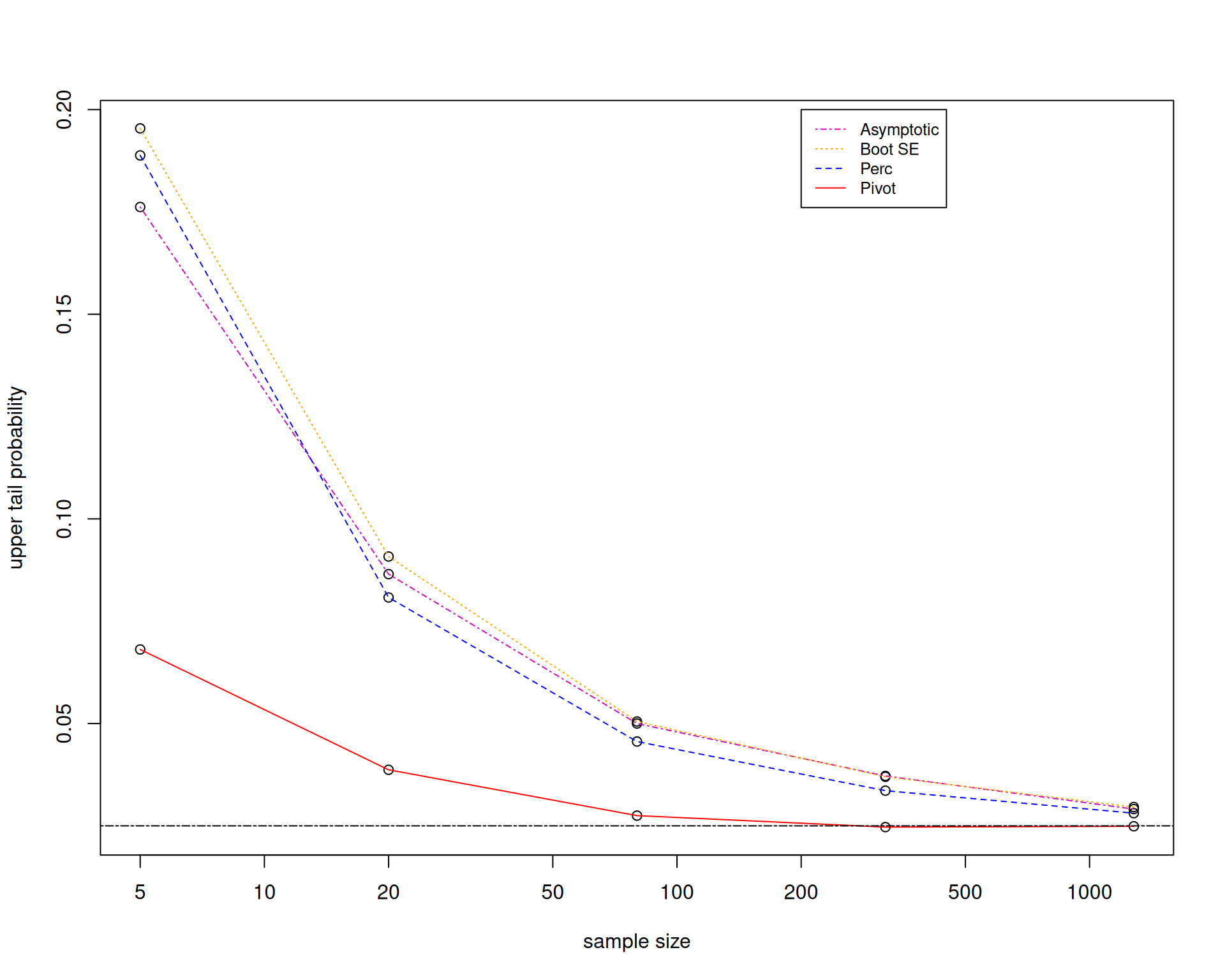
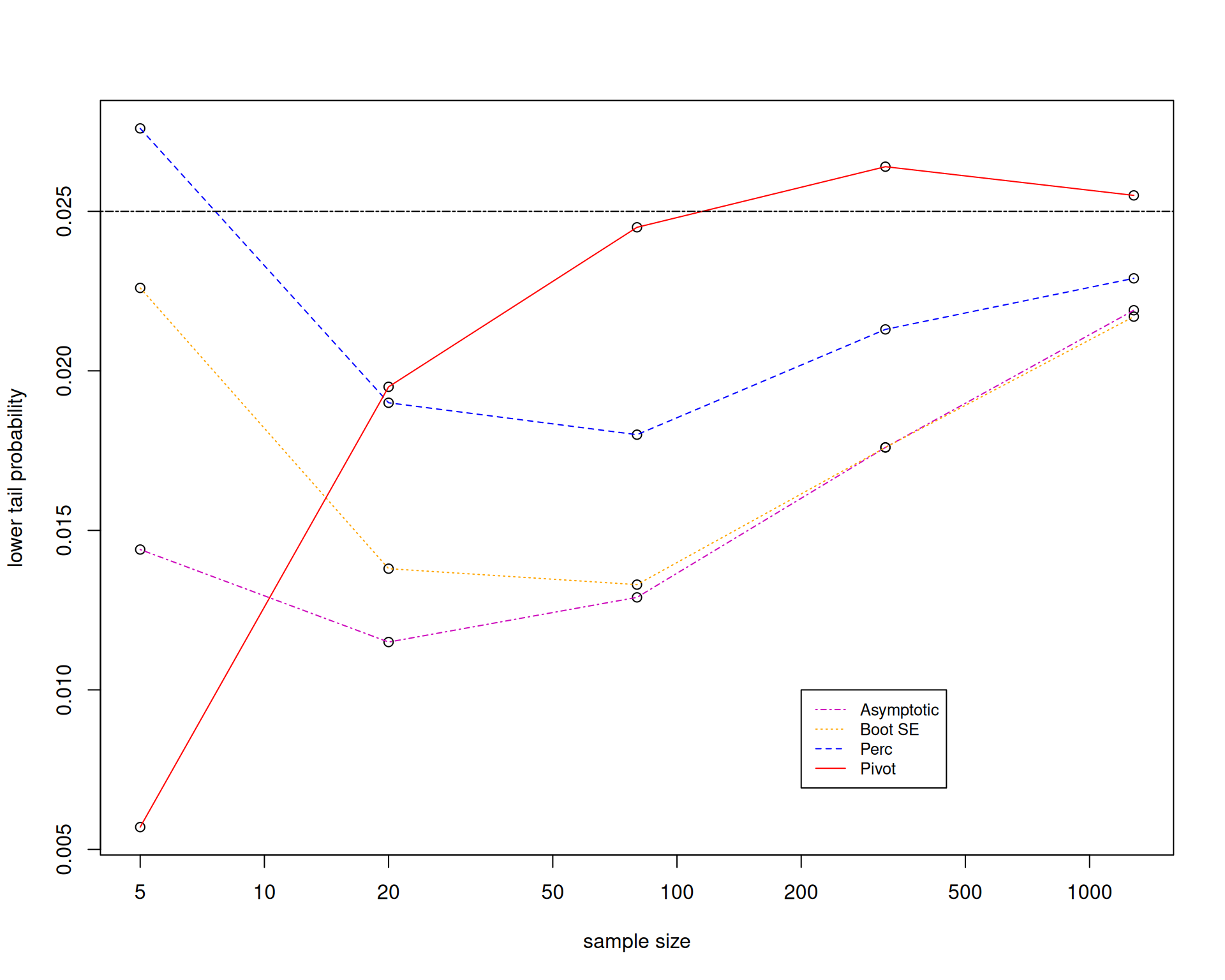
[1,] 0.43 0.89Simulation evidence for the bootstrap confidence intervals
Let us look at the performance of the different confidence intervals by using Monte Carlo simulation to figure out whether the bootstrap is working.
We will now focus on the case where \(X_1,\ldots,X_n\overset{\mathsf{IID}}{\sim} Exp\left(3\right)\).
The main recommendation is that it is really preferable to bootstrap an asymptotically pivotal statistic.
But the bootstrap pivotal confidence interval requires you to have a formula for the standard error, so that you can bootstrap the pivot.
This becomes complicated in higher dimensions, especially in regression settings.
You could do a bootstrap within a bootstrap. Bootstrap the standard error, then bootstrap the pivot. This is called the double bootstrap.
Therefore, it is still important to know how to derive formulas for standard errors to reduce computational time.
The bootstrap in regression settings
- You can implement the calculation of bootstrapped standard errors in regression settings using the
sandwichpackage. - It works after applying
lm(). - In regression settings, there are again multiple versions of the bootstrap. I talk about two versions.
- Pairs bootstrap: Resample with replacement every row of your spreadsheet. Thus, you can think of this as a version of the nonparametric bootstrap extended to the regression case.
- Residual bootstrap: Use the estimated regression for your sample, resample with replacement from the residuals, and generate the \(Y\)’s again taking \(X\)’s fixed. Thus, you can think of this as a mix of the parametric and nonparametric bootstrap.
- Pairs bootstrap works well even without correct specification. Residual bootstrap requires correct specification.
- Let us go back to the compensation-sales relationship. We reload the data once again.
dataset1 <- read.csv("sia1_ceo_comp.csv")
dataset2 <- read.csv("04_4m_exec_comp_2003.csv")
names(dataset1) <- c("Name", "Company", "Industry", "TotalCompMil",
                     "NetSalesMil", "Log10TotalComp")
names(dataset2) <- c("SalaryThou", "Name", "Company", "Industry",
                     "TotalCompMil")
execComp <- merge(dataset1, dataset2,
                  by=c("Name","Company", "Industry", "TotalCompMil"))
eCsub <- subset(execComp, (TotalCompMil>0 & NetSalesMil>0))(Intercept) NetSalesMil
3.76708 0.00017 (Intercept) NetSalesMil
(Intercept) 2.5e-02 -5.3e-07
NetSalesMil -5.3e-07 1.0e-10 (Intercept) NetSalesMil
(Intercept) 3.3e-02 -3.7e-06
NetSalesMil -3.7e-06 1.0e-09 (Intercept) NetSalesMil
(Intercept) 3.5e-02 -4.0e-06
NetSalesMil -4.0e-06 1.1e-09cbind(
"classical" = sqrt(diag(vcov(reg.comp))),
"heteroscedasticity-consistent" = sqrt(diag(vcovHC(reg.comp))),
"pairs bootstrap" = sqrt(diag(vcovBS(reg.comp, R = 999)))
) classical heteroscedasticity-consistent pairs bootstrap
(Intercept) 0.15728 1.8e-01 1.8e-01
NetSalesMil 0.00001 3.2e-05 3.2e-05 (Intercept) log(NetSalesMil)
-1.9 0.4 (Intercept) log(NetSalesMil)
(Intercept) 0.0124 -0.00163
log(NetSalesMil) -0.0016 0.00023 (Intercept) log(NetSalesMil)
(Intercept) 0.016 -0.00203
log(NetSalesMil) -0.002 0.00027 (Intercept) log(NetSalesMil)
(Intercept) 0.0144 -0.00186
log(NetSalesMil) -0.0019 0.00025cbind(
"classical" = sqrt(diag(vcov(reg.log.comp))),
"heteroscedasticity-consistent" = sqrt(diag(vcovHC(reg.log.comp))),
"pairs bootstrap" = sqrt(diag(vcovBS(reg.log.comp, R = 999)))
) classical heteroscedasticity-consistent pairs bootstrap
(Intercept) 0.111 0.125 0.121
log(NetSalesMil) 0.015 0.017 0.016- It was only shown very recently that the pairs bootstrap in the IID setting and the heteroscedasticity-consistent standard errors are asymptotically equivalent.
Things about the bootstrap left hanging
- How do I construct bootstrap pivotal confidence intervals? You have to search for a pivotal or more ikely an asymptotically pivotal statistic.
- What happens to the bootstrap if you are outside the IID setting? Then resampling with replacement may not be the best idea.
- How about bootstrap hypothesis tests? You have to take into account the claim under the null.